Here I show how to do some simple summary statistics with the dplyr package.

We will be using the followint packages:

library(lubridate)
library(dplyr)
library(readr)
library(ggplot2)

get DWD data

Files can be downloaded and unzipped by hand from https://opendata.dwd.de/climate_environment/CDC/observations_germany/climate/daily/kl/historical. Or you can use the following script:

data_dir = "data/dwd"
dir.create(data_dir)

urls <- c(Cottbus="https://opendata.dwd.de/climate_environment/CDC/observations_germany/climate/daily/kl/historical/tageswerte_KL_00880_18870101_20231231_hist.zip",
          Warnemünde="https://opendata.dwd.de/climate_environment/CDC/observations_germany/climate/daily/kl/historical/tageswerte_KL_04271_19470101_20231231_hist.zip",
          #Freiberg="https://opendata.dwd.de/climate_environment/CDC/observations_germany/climate/daily/kl/historical/tageswerte_KL_01441_19450701_19930430_hist.zip",
          #Stuttgart="https://opendata.dwd.de/climate_environment/CDC/observations_germany/climate/daily/kl/historical/tageswerte_KL_04927_19490801_19840731_hist.zip",
          "Garmisch-Patenkirchen"="https://opendata.dwd.de/climate_environment/CDC/observations_germany/climate/daily/kl/historical/tageswerte_KL_01550_19360101_20231231_hist.zip",
          Zugspitze="https://opendata.dwd.de/climate_environment/CDC/observations_germany/climate/daily/kl/historical/tageswerte_KL_05792_19000801_20231231_hist.zip")

for(url in urls){
  destfile = file.path(data_dir, basename(url))
  if(!file.exists(destfile)){
    download.file(url, destfile)
    unzip(destfile, exdir = data_dir)
  }
}

read data

We use the readr package to read the csv files:

data_files <- list.files(data_dir, pattern="produkt_klima_tag", full.names = T)

data <- read_delim(data_files, delim = ";", na = "-999", trim_ws = T)

We use list.files to list all files starting with “produkt_klima_tag” in the data directory. The read_delim function reads all files into a single R object. Stations can be identified by their STATIONS_ID in the dataset.

See what’s in the dataset:

data

## # A tibble: 153,294 × 19
##    STATIONS_ID MESS_DATUM  QN_3    FX    FM  QN_4   RSK  RSKF   SDK SHK_TAG
##          <dbl>      <dbl> <dbl> <dbl> <dbl> <dbl> <dbl> <dbl> <dbl>   <dbl>
##  1         880   18870101    NA    NA    NA     1   0       0    NA       0
##  2         880   18870102    NA    NA    NA     1   0       0    NA       0
##  3         880   18870103    NA    NA    NA     1   0       0    NA       0
##  4         880   18870104    NA    NA    NA     1   0       0    NA       0
##  5         880   18870105    NA    NA    NA     1   0       0    NA       0
##  6         880   18870106    NA    NA    NA     1   0       0    NA       0
##  7         880   18870107    NA    NA    NA     1   3.3     4    NA       4
##  8         880   18870108    NA    NA    NA     1   0       0    NA       4
##  9         880   18870109    NA    NA    NA     1   0       0    NA       4
## 10         880   18870110    NA    NA    NA     1   0       0    NA       4
## # ℹ 153,284 more rows
## # ℹ 9 more variables: NM <dbl>, VPM <dbl>, PM <dbl>, TMK <dbl>, UPM <dbl>,
## #   TXK <dbl>, TNK <dbl>, TGK <dbl>, eor <chr>

convert data

Convert date:

data <- data %>%
  mutate(MESS_DATUM = as.POSIXct(as.character(MESS_DATUM), format="%Y%m%d")) %>%
  mutate(STATIONS_ID = as.factor(STATIONS_ID))

The %>% notation and mutate function comes from the dplyr package.

Calculate yday and month:

data <- data %>%
  mutate(yday = yday(MESS_DATUM)) %>%
  mutate(month = month(MESS_DATUM))

The yday and month functions come from the lubridate package

Add station names:

stations <- tribble(
  ~STATION_NAME, ~STATIONS_ID,
  "Cottbus", "880",
  "Warnemünde", "4271",
  "Garmisch-Patenkirchen", "1550",
  "Zugspitze", "5792"
)

data <- data %>% left_join(stations)

plot some data

We plot data with the ggplot2 package:

data %>%
  ggplot() +
  aes(x=yday, y=TMK) +
  geom_point(size=0.1, alpha=0.1) +
  facet_wrap(STATION_NAME~.)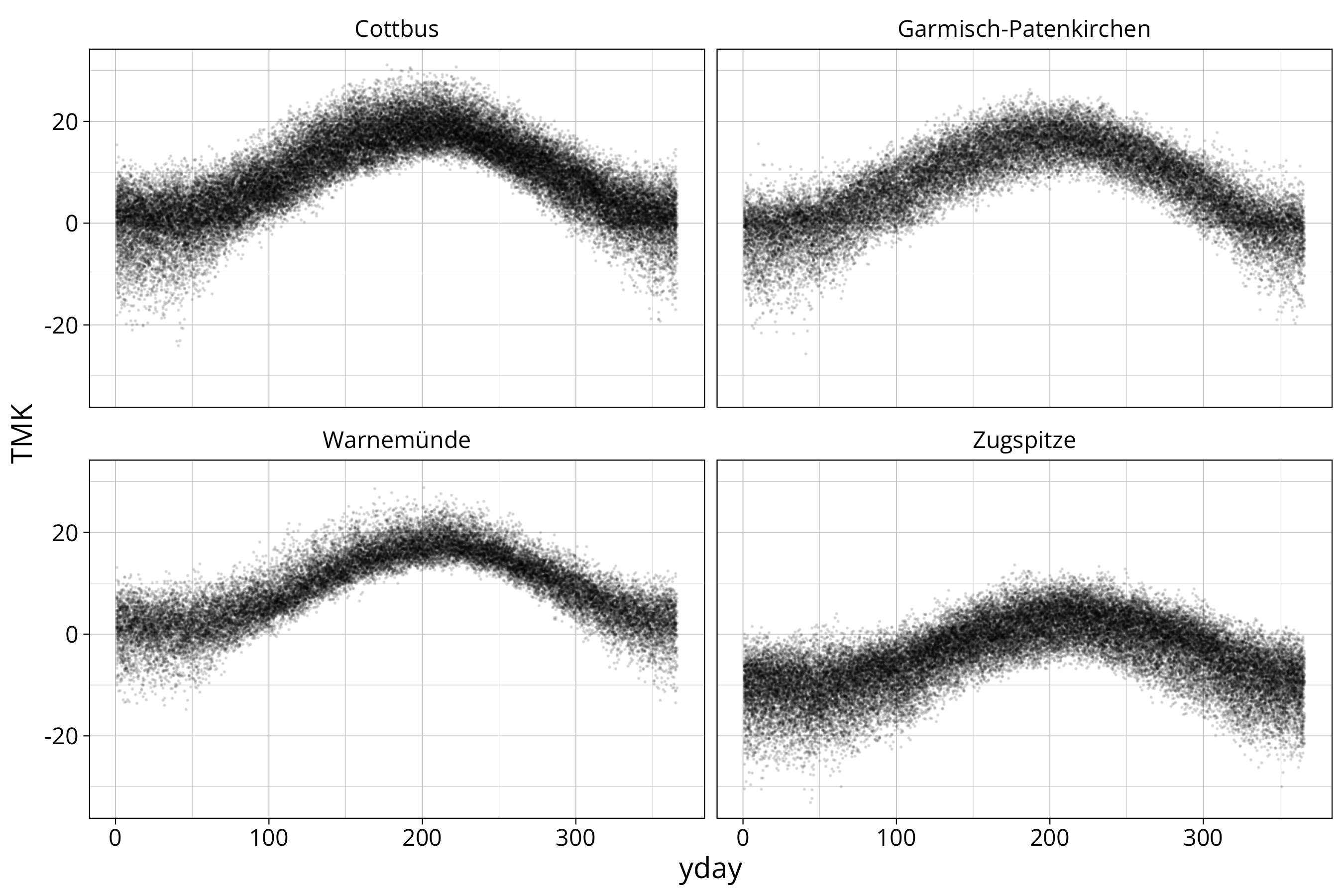

plot of chunk plot temperature data facet_wrap creates a single graph for each station.

calculate mean for month

longterm_average_month <- data %>%
  group_by(STATION_NAME, month) %>%
  summarise("temp longterm average" = mean(TMK, na.rm=T), "rain longterm average" = mean(RSK, na.rm=T))

With group_by and summarise we again use functions from the dplyr package. The procedure is to form multiple subsets of the dataset with group_by and then calculate the summary statistics for those subsets. We group by STATION_NAME and month.

In the next plot we put all stations into one graph:

longterm_average_month %>%
  ggplot() +
  aes(x=month, y=`temp longterm average`, col=STATION_NAME, group=STATION_NAME) +
  geom_line()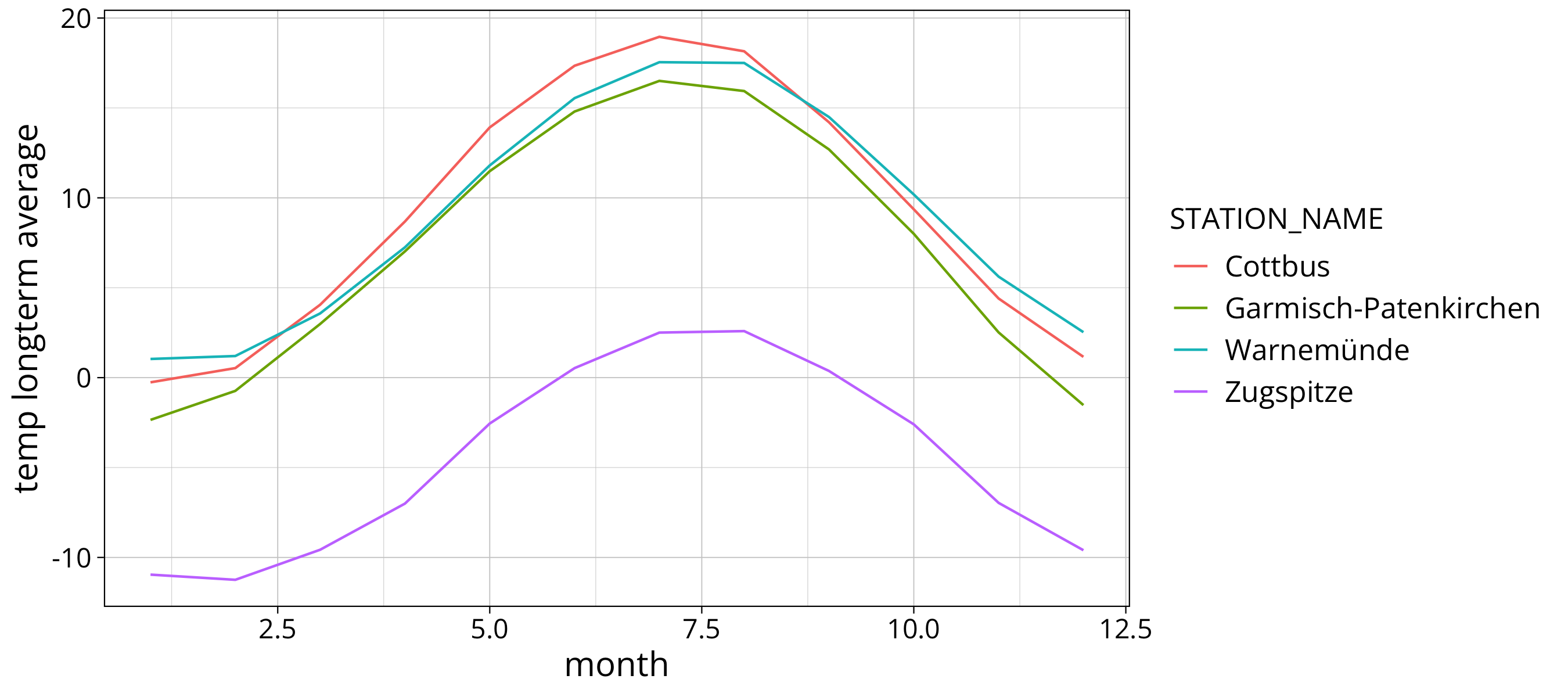

plot of chunk plot temp monthly average

calculate mean for yday

longterm_average_yday <- data %>%
  group_by(STATION_NAME, yday) %>%
  summarise("temp longterm average" = mean(TMK, na.rm=T), "rain longterm average" = mean(RSK, na.rm=T))

data %>%
  ggplot() +
  aes(x=yday, y=TMK) +
  geom_point(size=0.1, alpha=0.1) +
  geom_line(aes(x=yday, y=`temp longterm average`), data=longterm_average_yday, col="red") +
  facet_wrap(STATION_NAME~.)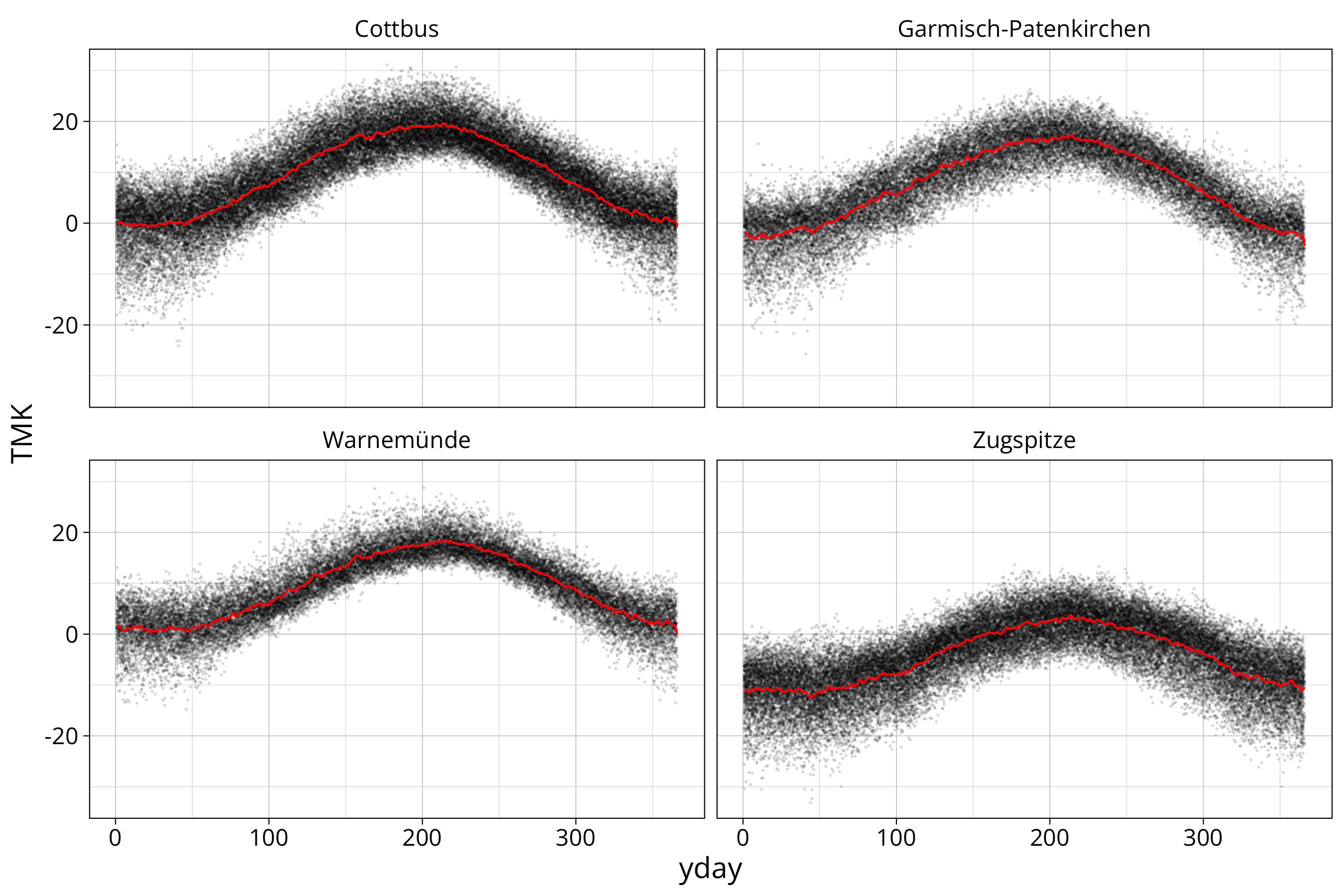

plot of chunk plot yday average with scatterplot

precipitation

data %>%
  ggplot() +
  aes(x=yday, y=RSK) +
  scale_y_continuous(trans="log10") +
  geom_point(size=0.1, alpha=0.1) +
  facet_wrap(STATION_NAME~.)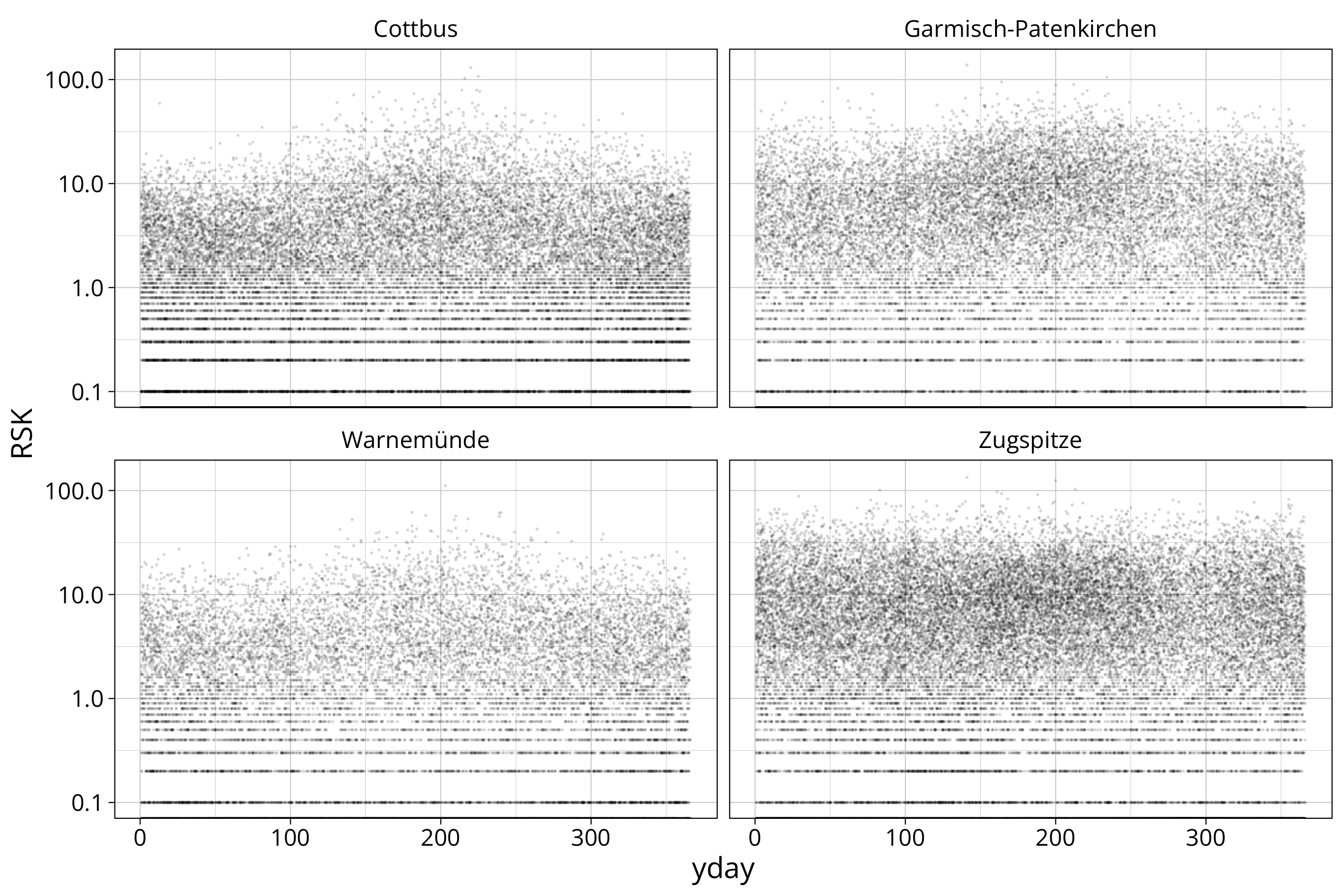

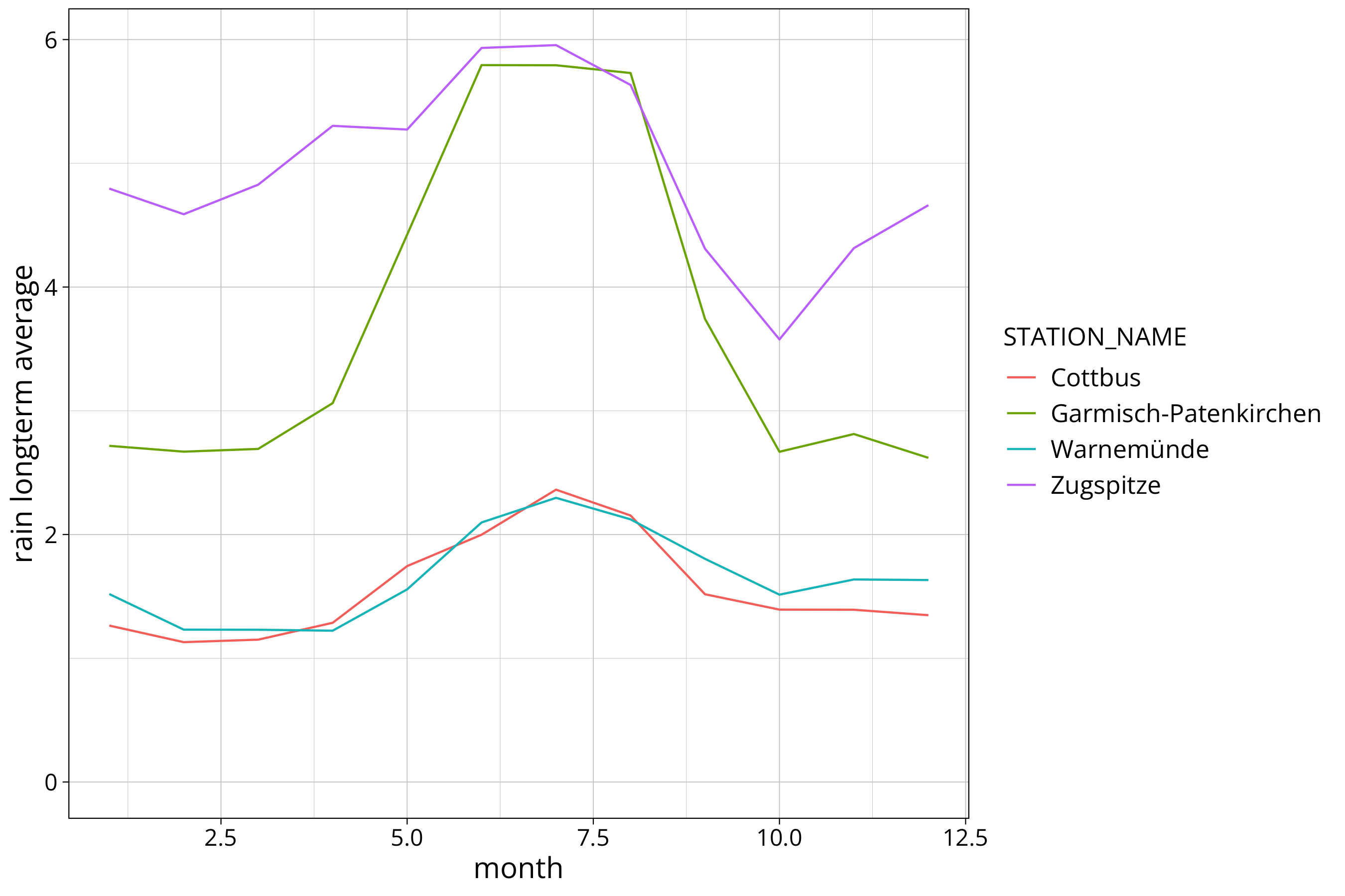
plot of chunk rain scatterplot

longterm_average_month %>%
  ggplot() +
  aes(x=month, y=`rain longterm average`, col=STATION_NAME, group=STATION_NAME) +
  #scale_y_continuous(trans="log10") +
  geom_line()

plot of chunk rain monthly average plot