The “NASA Global Precipitation Measurement” (GPM) is a sattelite data product to estimate precipitation on a global scale. More precise we will be using the “Integrated Multi-satellitE Retrievals for GPM” (IMERG) data product which merges, intercalibrates and interpolates data from different satellites. It brings together microwave measurements and IR measurements and calibrates against gauge measurements on the ground. It also brings together data from low-earth-orbit satellites with geosynchronous-earth-orbit satellite data. The low-earth-orbit (leo) satellites can’t measure continuously in one spot but rather have a return period with temporal blindspots in between. Geosynchronous-Earth-orbit (geo) satellites can’t take the passive microwave (PMW) measurements that are possible with leo satellites. To get global coverage without temporal gaps morphing and interpolation between the different data sources is done.

The data product uses data from different satellite programs and generations. Most of them are not under the control of the GPM program. GPM rather uses the best data available from other programs. More infos about the data product can be found in the product description document. It can be downloaded from different sources. Here is a summary on how to download.

creating an account and credential file

To download gpm data you have to create an EarthData account and authorise the GESDISC application in your newly created account.

We have to save the credentials to your account into a .netrc file. This file then can be used by wget or R. Here are two sources on how to do that:

• save your earthdata account credentials in a file
• Instructions on how to download data with wget

There is also a specific descriptions about how to access data with R:

• How to access data with R.
• OPeNDAP access with R

global dataset (no subsetting)

The global dataset can be downloaded from the online archive at https://gpm1.gesdisc.eosdis.nasa.gov/data/GPM_L3/GPM_3IMERGDF.06/. This page basically works like an ftp server where you find a file for every day in the measuring period. You can download those files similar to the way shown for the subregion datasets below.

subregion dataset with OPeNDAP

Data for selected regions can be downloaded via the OPeNDAP data selection form. This tool shows you a url with all the options that you chose. You can take that url and automate the download for your specific region. The only trick is that you have to add the file format into the url as shown below.

You can select variables by ticking the checkbox beside the variable name. In the input fields you put the range of time and the latitude and longitude you want to download. The inputs work with the scheme [from:step:to]. Since the dataset is produced in 0.1° intervals, longitude ranges from 0 to 3599 (\(360\cdot 10-1\)) and latitude from 0 to 1799 (\(180\cdot 10-1\)). Hence to select a subset from longitude 90 to 120 you write the input as [900:1:1200]. If you want a resulution of only 1° instead of 0.1° you can set the input to [900:10:120].

The following shows how to use the url as a template for assembling a download url from latitude and longitude range and a date

library(stringr)
library(lubridate)

fileformat = "nc4"
# other options are "nc", "ascii", "dap" and "covjson"

min_longitude = 0 *10
max_longitude = 3599
lon_aggregation = 10

min_latitude = 0 *10
max_latitude = 1799
lat_aggregation = lon_aggregation

date = as.Date("2010-02-17")

year = year(date)
month = str_pad(month(date), width=2, pad="0")
day = str_pad(day(date), width=2, pad="0")

url <- str_glue("https://gpm1.gesdisc.eosdis.nasa.gov/opendap/GPM_L3/GPM_3IMERGDF.06/{year}/{month}/3B-DAY.MS.MRG.3IMERG.{year}{month}{day}-S000000-E235959.V06.nc4.{fileformat}?precipitationCal[0:1:0][{min_longitude}:{lon_aggregation}:{max_longitude}][{min_latitude}:{lat_aggregation}:{max_latitude}],lat[{min_latitude}:{lat_aggregation}:{max_latitude}],lon[{min_longitude}:{lon_aggregation}:{max_longitude}],time[0:1:0]")

download_folder = "../data/gpm"

destfilename = basename(url) %>% str_extract("[^?]*") %>% file.path(download_folder, .)

We can now download the data with the GET() function of the httr package. We give the function the paths to the .netrc file we created earlier.

library(httr)
netrc_path <- "../data/gpm/.netrc"
cookie_path <- "../data/gpm/.urs_cookies"
downloaded_file_path <- "../data/gpm"

set_config(config(followlocation=1,netrc=1,netrc_file=netrc_path,cookie=cookie_path,cookiefile=cookie_path,cookiejar=cookie_path))

httr::GET(url = url, write_disk(destfilename, overwrite = TRUE))

If we get a response status 200 all went well. Status 400 means that something is wrong with our credentials.

opendapr R package

A more convenient way of downloading opendap data is the opendapr package. To install it we have to execute the following:

# install.packages("devtools")
devtools::install_github("ptaconet/opendapr")

Let’s load the package and start working with it:

library(opendapr)

We have to set our credentials and call the odr_login() function:

username <- "my_username"
password <- "my_password"

log <- odr_login(credentials=c(username, password), source = "earthdata")

In order to query data we need a bounding box. We will use the getbb() function of the osmdata package which enables us to get bounding boxes by searching for a country name, county name or city name for example.

library(osmdata)
library(sf)

Brandenburg <- getbb("Brandenburg", featuretype="county", format_out = "sf_polygon", limit=1)$multipolygon

plot(Brandenburg)

roi <- Brandenburg %>%
  st_bbox() %>%
  st_as_sfc() %>%
  st_as_sf()

lines(roi)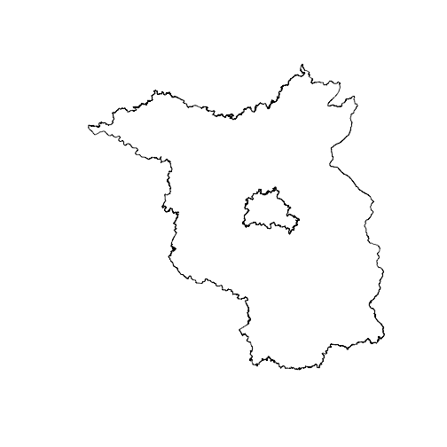

As you see we have to convert the bounding box multple times to get it in the right format that the odr_get_url() function of the opendapr package requires. We also have to define a time range:

time_range <- as.Date(c("2017-01-01","2017-01-03"))

urls <- odr_get_url("GPM_3IMERGDF.06", variables = "precipitationCal", roi = roi, time_range = time_range)

Now we have the urls that we can use to download data with the odr_download_data() function:

odr_download_data(urls)

plot data

To validate that we can read the data we just downloaded we use the stars and the ncmeta package. According to my tests the read_ncdf() function is the only one that reads the netCDF files with latitude and longitude in the right order. Functions from the terra or raster package don’t realize that latitude and longitude have to be read in reverse order in this case. QGis also reads the files rotated.

First let’s test the global file:

library(stars)
library(ncmeta)

nc4 <- read_ncdf(destfilename, var="precipitationCal") %>%
  st_set_crs("+proj=longlat +datum=WGS84")

Note that we set the coordinate system to WGS84 since the file does not contain a crs.

We now can plot the dataset:

plot(nc4)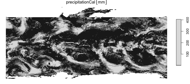

A more convenient plotting function can be found in the tmap package:

library(tmap)
tmap_mode("plot")

# load dataset with country boundaries
data("World")

tm_shape(nc4) +
  tm_graticules() +
  tm_raster("precipitationCal", breaks=c(0,1,2,5,10,500), legend.is.portrait = F) +
  tm_shape(World) +
  tm_borders() +
  tm_layout(legend.outside=T, legend.outside.position = "bottom", legend.position = c("center", "top"))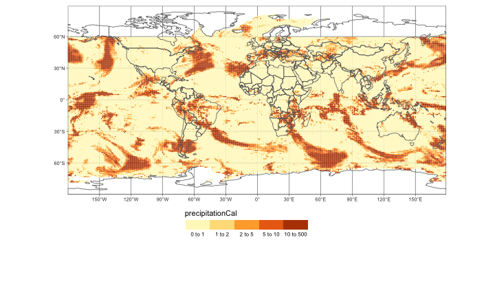 

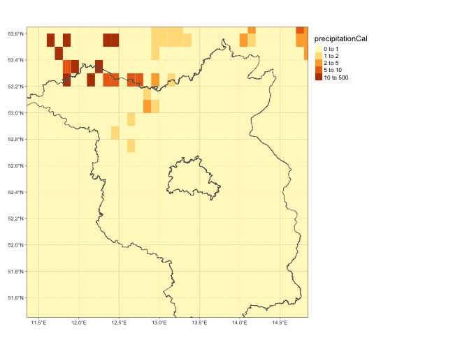
Next we work with the subregion dataset that we downloaded with the opendapr package:

nc4_opendapr <- read_ncdf(urls$destfile[1], var="precipitationCal") %>%
  st_set_crs("+proj=longlat +datum=WGS84")

The bounding box of the downloaded file is slightly different from what we set in the bounding box:

st_bbox(nc4_opendapr)

##  xmin  ymin  xmax  ymax 
## 11.35 51.45 14.85 53.65

st_bbox(Brandenburg)

##  xmin  ymin  xmax  ymax 
## 11.27 51.36 14.77 53.56

Plot with tmap:

tm_shape(nc4_opendapr) +
  tm_graticules() +
  tm_raster("precipitationCal", breaks=c(0,1,2,5,10,500)) +
  tm_shape(Brandenburg) +
  tm_borders() +
  tm_layout(legend.outside=T)