In this post I will demonstrate that a periodic signal can be fitted with a linear model using a sine and cosine transform on the input signal.

We will be using the following packages:

library(lubridate)
library(dplyr)
library(readr)
library(stringr)
library(ggplot2)
library(knitr)

We will be using data from the German weather service (DWD) which we can download in the following way:

dir.create("data/dwd")
destfile="data/dwd/stundenwerte_TU_03987_18930101_20231231_hist.zip"
if(!file.exists(destfile)){
  download.file("https://opendata.dwd.de/climate_environment/CDC/observations_germany/climate/hourly/air_temperature/historical/stundenwerte_TU_03987_18930101_20231231_hist.zip", destfile)
  unzip("data/dwd/stundenwerte_TU_03987_18930101_20231231_hist.zip", exdir = "data/dwd/Görlitz")
}

The data is in csv format and can be read with read_delim from the readr package:

temp_data <- read_delim("data/dwd/Görlitz/produkt_tu_stunde_18930101_20231231_03987.txt", delim = ";", na = "-999", trim_ws = T) %>%
  mutate(MESS_DATUM = as.POSIXct(as.character(MESS_DATUM), format="%Y%m%d%H")) %>%
  select(MESS_DATUM, TEMP=TT_TU) %>%
  mutate(yday = yday(MESS_DATUM)) %>%
  mutate(yday_rad = yday/365*2*pi) %>%
  na.omit()

We add the yday column by using the yday function of the lubridate package on MESS_DATUM. We then transform yday to radians of the 365 day yearly cycle:

\[yday_{rad} = \frac{yday}{365}\cdot 2\pi\]

This way we can use it directly in the sin and cos functions we will be using later.

Let’s dive right in by calculating the first linear model. Yo may be familiar to using the log transform on the input variable to fit log distributed data. You also can use the cos or sin functions to transform the input variable. Since the input signal also can be phase shifted we have to use a combination of sin and cos. Hence we define the model in the following way:

temp_sin_model <- lm(TEMP ~ sin(yday_rad) + cos(yday_rad), data=temp_data)

We add the predicted values and residuals to the original data frame:

temp_data$sin_model_prediction <- predict(temp_sin_model)
temp_data$sin_model_residuals <- residuals(temp_sin_model)

This way we can add the prediction to a scatterplot of the data:

temp_data %>%
  ggplot() +
  aes(x=yday, y=TEMP) +
  geom_point(size=0.01, alpha=0.05) +
  geom_line(aes(y=sin_model_prediction), col="red", linewidth=1.5)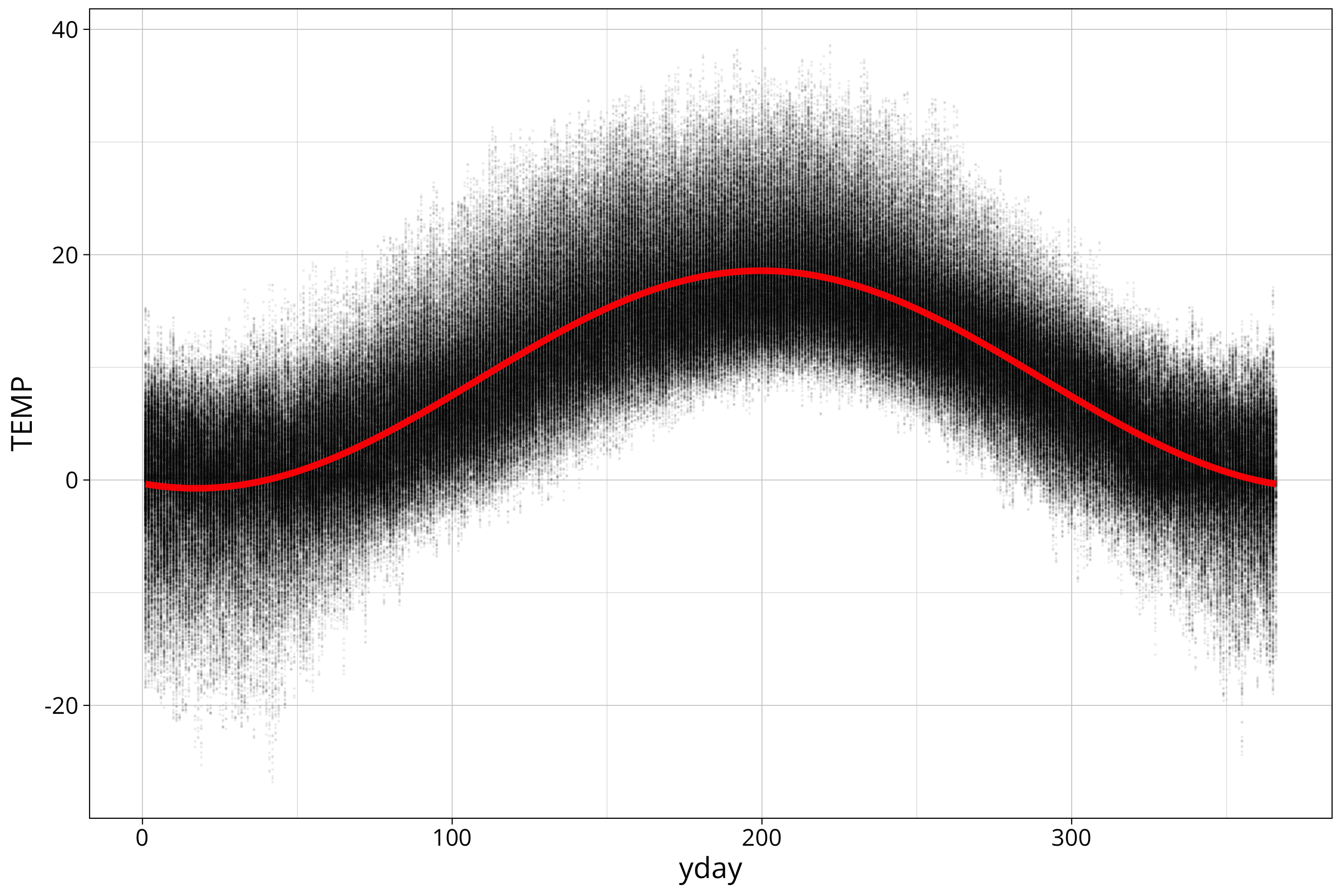

plot of chunk temp sin model with data

You can see that we have a pretty good fit. Let’s look at the residuals to verify that:

temp_data %>%
  ggplot() +
  aes(x=yday, y=sin_model_residuals) +
  geom_point(size=0.01, alpha=0.05) +
  geom_hline(yintercept = 0, col="red", linewidth=2) +
  geom_smooth()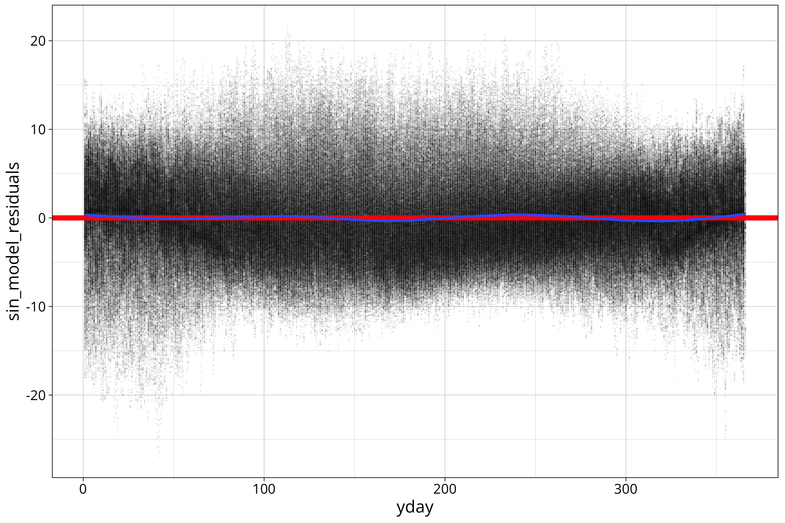

plot of chunk residuals of temp sin model

I added a geom_smooth() to the plot which fits a loess function to the data. This helps to identify remaining variation in the mean of the residuals. You can see a slight wobble in the loess which indicates that there is a weak second frequency in the data. But I consider it too weak to take into account.

For now we will ignore that the distribution around the mean is not constant. There are other methods of finding residual oscillations in the data like the ACF function. We will not deal with that here.

calculate phase shift

An arbitrary cosine signal can be described in two ways:

\[A \cdot cos(\omega t + \varphi) = B \cdot cos(\omega t) + C \cdot sin(\omega t)\]

where on the left side we have \(A\), which is is the amplitude of the oscillation and \(\varphi\), which is the phase shift. \(\omega\) is the angular frequency.

On the right side we have the factors \(B\) and \(C\) which correspond to \(A\) in the following way:

\[A = \sqrt{B^2+C^2}\]

\(\varphi\) is related as follows:

\[\varphi=atan\left(\frac{B}{C}\right)\]

R has an atan2() function which takes into account the signs of both arguments to determine the correct quadrant of the resulting angle.

This way we can extract the following metrics:

intercept   <- temp_sin_model$coefficients[1] %>% unname
sin_factor  <- temp_sin_model$coefficients[2] %>% unname
cos_factor  <- temp_sin_model$coefficients[3] %>% unname
amplitude   <- sqrt(sin_factor^2 + cos_factor^2)
phase_angle <- (atan2(sin_factor, cos_factor)/(2*pi)*365) %% 365

The phase angle is transformed back to days in the 365 day cycle.

Let’s show the phase angle in a plot:

temp_data %>%
  ggplot() +
  aes(x=yday, y=TEMP) +
  geom_point(size=0.01, alpha=0.05) +
  geom_line(aes(y=sin_model_prediction), col="red", linewidth=1.5) +
  geom_vline(xintercept = phase_angle, col="red", linetype=2) +
  geom_vline(xintercept = phase_angle-365/2, col="orange", linetype=2)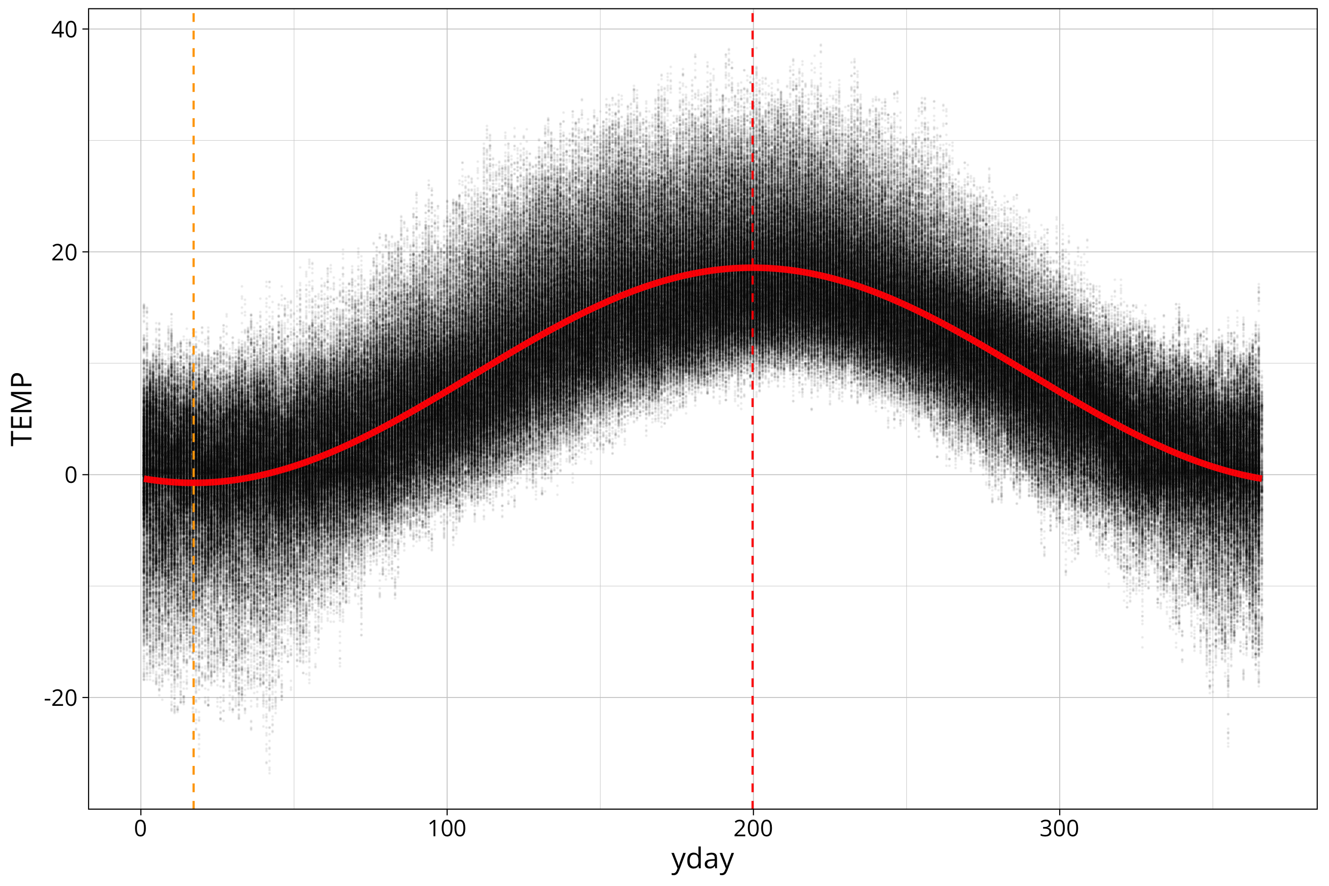

plot of chunk show pahse shift on data plot The orange line shows the minimum of the sine curve.

fit sine models with additional subfrequencies

Not every signal can be described by a single sine wave. We can easily add additional subfrequencies to the linear model.

To demonstrate this we use solar radiation data from the same station. This can be downloaded as followed:

destfile = "data/dwd/stundenwerte_ST_03987_row.zip"
if(!file.exists(destfile)){
  download.file("https://opendata.dwd.de/climate_environment/CDC/observations_germany/climate/hourly/solar/stundenwerte_ST_03987_row.zip", destfile)
  unzip("data/dwd/stundenwerte_ST_03987_row.zip", exdir = "data/dwd/Görlitz")
}

We read the data the same way as the temperature data:

solar_data <- read_delim("data/dwd/Görlitz/produkt_st_stunde_19451231_20240331_03987.txt", delim=";", na="-999", col_types = "ccnnnnnncc", trim_ws = T) %>%
  mutate(MESS_DATUM = as.POSIXct(as.character(MESS_DATUM), format="%Y%m%d%H:%M")) %>%
  mutate(MESS_DATUM_WOZ = as.POSIXct(as.character(MESS_DATUM_WOZ), format="%Y%m%d%H:%M")) %>%
  mutate(yday = yday(MESS_DATUM)) %>%
  mutate(yday_rad = yday/365*2*pi) %>%
  mutate(hour = hour(MESS_DATUM_WOZ)) %>%
  filter(hour == 12)

We filter data at solar noon (MESS_DATUM_WOZ == 12). WOZ is the real local time (Wahre Ortszeit in German).

We extract the max and mean for every day of the yearly cycle for all years in the data set:

max_solar <- solar_data  %>%
  group_by(yday, yday_rad) %>%
  summarise(max_solar = max(FG_LBERG, na.rm=T), mean_solar = mean(FG_LBERG, na.rm=T)) %>%
  na.omit

The syntax is from the dplyr package. We use group_by() to group the data by yday and then use the summarise() function to calculate the mean and max of the radiation data. Finally we get rid of observations with missing data using the na.omit function.

To fit a sine model to the data we use the same syntax as for the temperature model:

max_solar_sin_model <- lm(max_solar ~ sin(yday_rad) + cos(yday_rad), data=max_solar)

max_solar$max_solar_sin_model_prediction <- predict(max_solar_sin_model)
max_solar$max_solar_sin_model_residuals <- residuals(max_solar_sin_model)

The next plot shows all data in the background and the maximum for every day in the year highlighted as solid dots. We can see that the fitted sine wave does not describe the data perfectly.

max_solar %>%
  ggplot() +
  aes(x=yday, y=max_solar) +
  scale_color_viridis_c() +
  geom_point(size=.01, alpha=0.1, aes(x=yday, y=FG_LBERG), data=solar_data) +
  geom_line(aes(y=max_solar_sin_model_prediction), col="green", lwd=1.5) +
  geom_point(size=.1, col="black")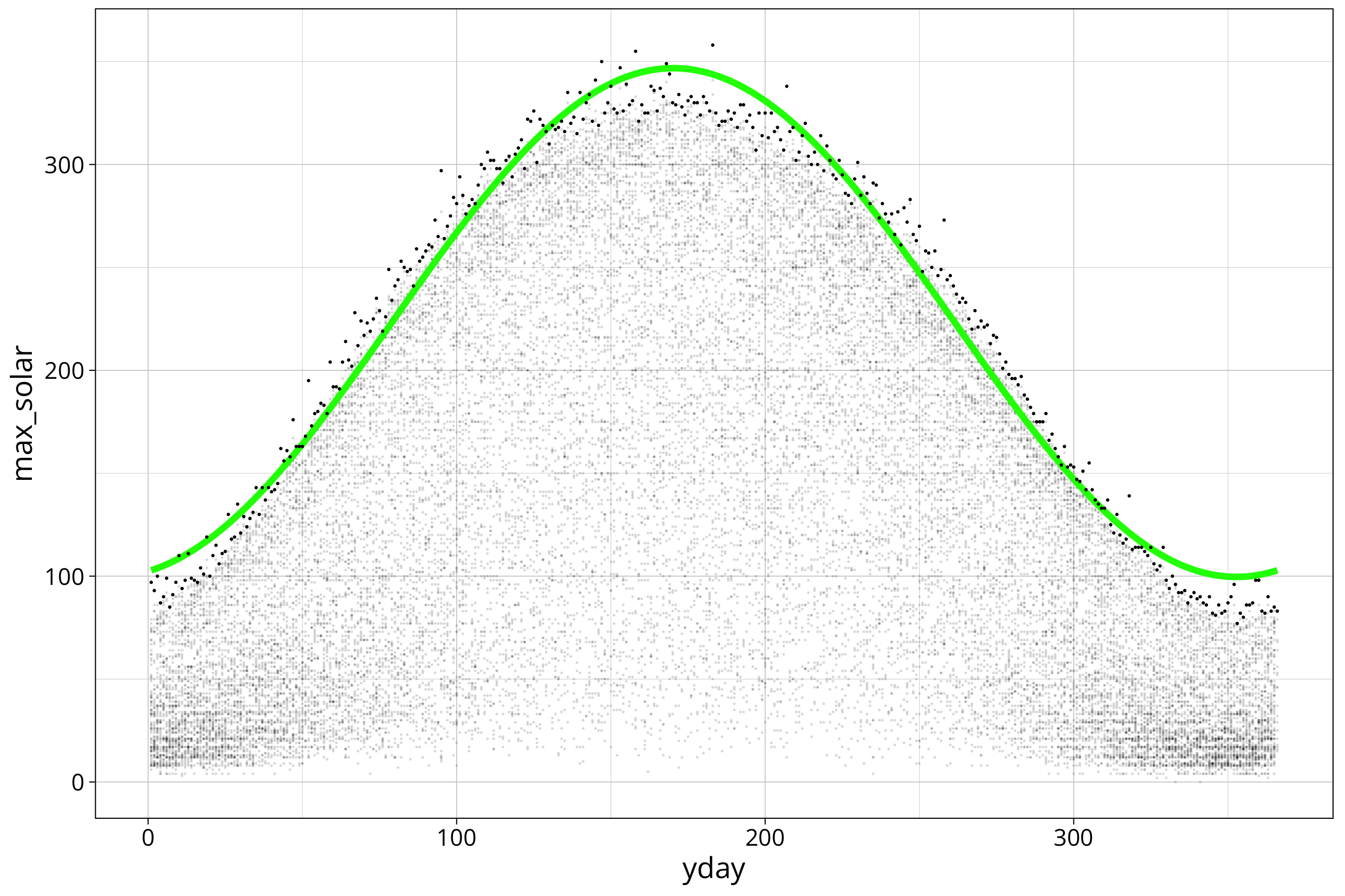

plot of chunk max solar sin model plot with data

Note that there are wavy patterns in the scatterplot that probably derive from the measuerement procedure. We will not deal with that.

If we plot the residuals we can clearly see that they contain an additional frequency of two times the yearly cycle.

max_solar %>%
  ggplot() +
  aes(x=yday, y=max_solar_sin_model_residuals) +
  geom_point()

plot of chunk max solar sin model residuals

To improve the fitting we can introduce additional subfrequencies into the model:

max_solar_sin3_model <- 
  lm(data=max_solar,
      max_solar ~  sin(yday_rad)   + cos(yday_rad) +
                   sin(2*yday_rad) + cos(2*yday_rad) +
                   sin(3*yday_rad) + cos(3*yday_rad)
  )

max_solar$max_solar_sin3_model_prediction <- predict(max_solar_sin3_model)
max_solar$max_solar_sin3_model_residuals <- residuals(max_solar_sin3_model)
max_solar_sin3_model$max_yday <- max_solar$yday[which.max(max_solar$max_solar_sin3_model_prediction)]

The anova (analysis of variance) table shows us that sin(2*yday_rad) and cos(2*yday_rad) frequencies are calculated as significant, while the sin(3*yday_rad) and cos(3*yday_rad) are not:

anova(max_solar_sin3_model)

## Analysis of Variance Table
## 
## Response: max_solar
##                    Df  Sum Sq Mean Sq    F value    Pr(>F)    
## sin(yday_rad)       1  123387  123387  2261.4284 < 2.2e-16 ***
## cos(yday_rad)       1 2726979 2726979 49979.8885 < 2.2e-16 ***
## sin(2 * yday_rad)   1    2179    2179    39.9384 7.771e-10 ***
## cos(2 * yday_rad)   1   39664   39664   726.9600 < 2.2e-16 ***
## sin(3 * yday_rad)   1       1       1     0.0099    0.9208    
## cos(3 * yday_rad)   1      52      52     0.9464    0.3313    
## Residuals         359   19588      55                         
## ---
## Signif. codes:  0 '***' 0.001 '**' 0.01 '*' 0.05 '.' 0.1 ' ' 1

We therefore could remove the third frequency from the model.

Let’s fit the same model to the mean radiation that we calculated earlier:

mean_solar_sin3_model <-  
  lm(data=max_solar,
    mean_solar ~  sin(yday_rad)   + cos(yday_rad) +
                  sin(2*yday_rad) + cos(2*yday_rad) +
                  sin(3*yday_rad) + cos(3*yday_rad) 
  )

max_solar$mean_solar_sin3_model_prediction <- predict(mean_solar_sin3_model)
max_solar$mean_solar_sin3_model_residuals <- residuals(mean_solar_sin3_model)
mean_solar_sin3_model$max_mean_yday <- max_solar$yday[which.max(max_solar$mean_solar_sin3_model_prediction)]

Since subfrequencies can have different phase shift to the main frequency we calculate the maximum of the model as a substitute for the overall phase shift. We will be using that later.

A look into the anova table shows us that here the third frequency is also significant:

anova(mean_solar_sin3_model)

## Analysis of Variance Table
## 
## Response: mean_solar
##                    Df Sum Sq Mean Sq    F value    Pr(>F)    
## sin(yday_rad)       1   6085    6085  1401.7994 < 2.2e-16 ***
## cos(yday_rad)       1 266936  266936 61495.9238 < 2.2e-16 ***
## sin(2 * yday_rad)   1     34      34     7.9069  0.005195 ** 
## cos(2 * yday_rad)   1    256     256    58.8912 1.589e-13 ***
## sin(3 * yday_rad)   1      3       3     0.7951  0.373160    
## cos(3 * yday_rad)   1    368     368    84.7889 < 2.2e-16 ***
## Residuals         359   1558       4                         
## ---
## Signif. codes:  0 '***' 0.001 '**' 0.01 '*' 0.05 '.' 0.1 ' ' 1

To show all data and fitted models together we plot the following:

max_solar %>%
  ggplot() +
  aes(x=yday, y=max_solar) +
  scale_color_viridis_c() +
  geom_point(size=.01, alpha=0.1, aes(x=yday, y=FG_LBERG), data=solar_data) +
  geom_line(aes(y=max_solar_sin3_model_prediction), col="green", lwd=1.5) +
  geom_point(size=.1, col="black") +
  geom_line(aes(y=mean_solar_sin3_model_prediction), col="orange", lwd=1.5) +
  geom_point(aes(y=mean_solar), size=.1, col="red")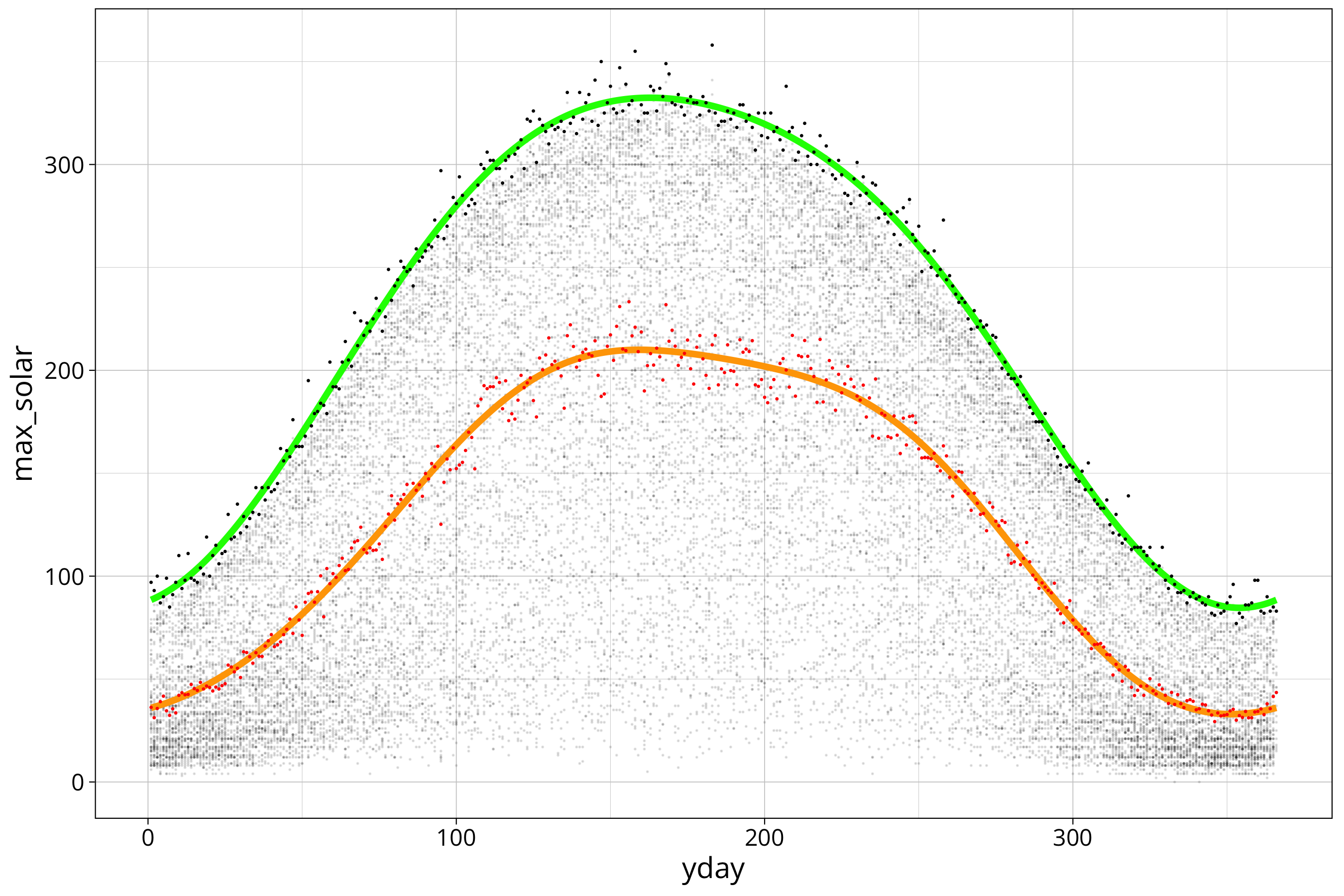

plot of chunk max solar sin3 fit

Red dots and the orange curve are the mean radiation data. We can see that both models fit the data quite good.

Again let’s look at the residuals:

max_solar %>%
  ggplot() +
  aes(x=yday, y=max_solar_sin3_model_residuals) +
  geom_point() +
  geom_hline(yintercept = 0, col="green", lwd=1.5) +
  geom_smooth()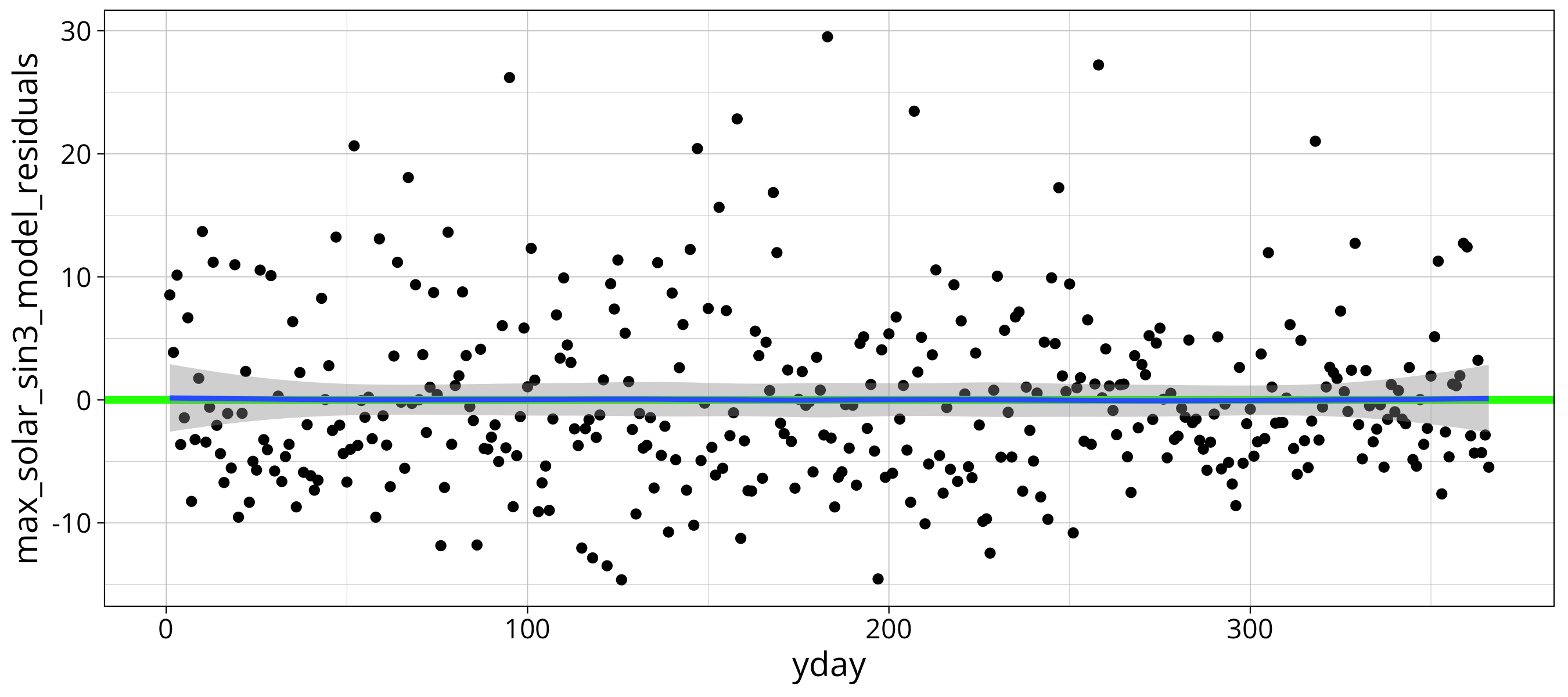

plot of chunk max solar sin3 model residuals

By checking the overlayed loess function we see that there is no significant residual frequency in the residuals. The same is true if the plot the residuals of the mean model.

compare phase shift

To compare the phase shift between the radiation data model and the temperature model we plot both functions into the same plot:

temp_data %>%
  ggplot() +
  aes(x=yday, y=TEMP) +
  
  geom_line(aes(y=sin_model_prediction), col="red", linewidth=1) +
  geom_line(aes(y = (max_solar_sin3_model_prediction-100)/10), data = max_solar, col = "green") +
  geom_line(aes(y = (mean_solar_sin3_model_prediction-100)/10), data = max_solar, col = "orange") +
  
  geom_vline(xintercept = phase_angle, col="red", linetype=2) +
  geom_vline(xintercept = max_solar_sin3_model$max_yday, col="green", linetype=2) +
  geom_vline(xintercept = mean_solar_sin3_model$max_mean_yday, col="orange", linetype=2) +
  
  scale_y_continuous(
    name = "temperature [°C]",
    sec.axis = sec_axis(~ .*10+100, name = "radiation [J/cm^2]")
  )

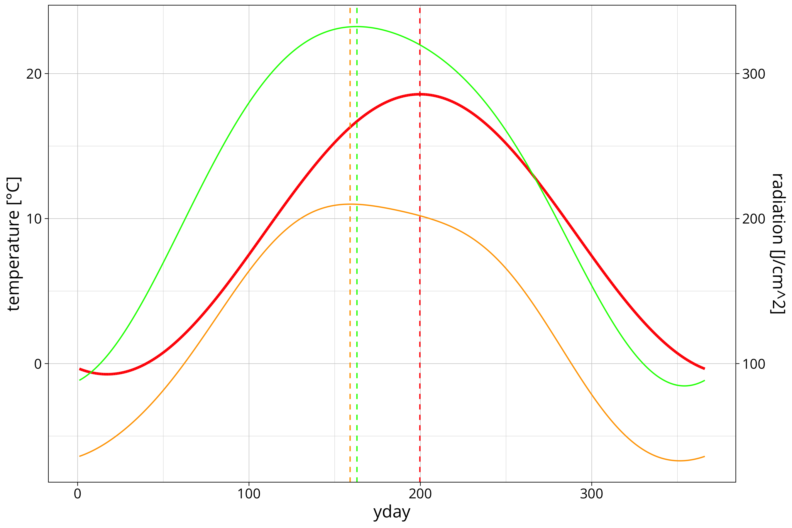
plot of chunk combined plot with radiation and temperature curves

We can see that the maximum of the mean radiation fitting is a bit later than the maximum radiation. The maximum temperature is a good 36 days behind the maximum of radiation. This is only logical since radiation is the driver of the atmospheric warming and the whole landmass/water body/atmosphere system has some heat capacity to buffer the heating process.

We can visualize the lag in the radiation and temperature curve in an interesting way. For that we make predictions of all our models for a single yearly cycle:

ydays <- 1:365
yday_rad <- ydays/365*2*pi
year_prediction <- tibble(yday=ydays,
  temp=predict(temp_sin_model, list(yday_rad=yday_rad)), 
  max_solar = predict(max_solar_sin3_model, list(yday_rad=yday_rad)),
  mean_solar = predict(mean_solar_sin3_model, list(yday_rad=yday_rad)),
  date = as.Date("2010-01-01")+days(yday-1),
  month=month(date), 
  mday=mday(date),
  first_of_month = if_else(mday==1, month, NA)
)

The plot is then generated as followed:

year_prediction %>%
  ggplot() +
  aes(y=temp, x=max_solar, col=yday) +
  scale_color_gradientn(colours = rainbow(10), na.value=NA) +
  geom_path(lwd=2) +
  geom_point(aes(col=first_of_month), size=4) +
  geom_label(aes(label=month.abb[first_of_month]), col="black")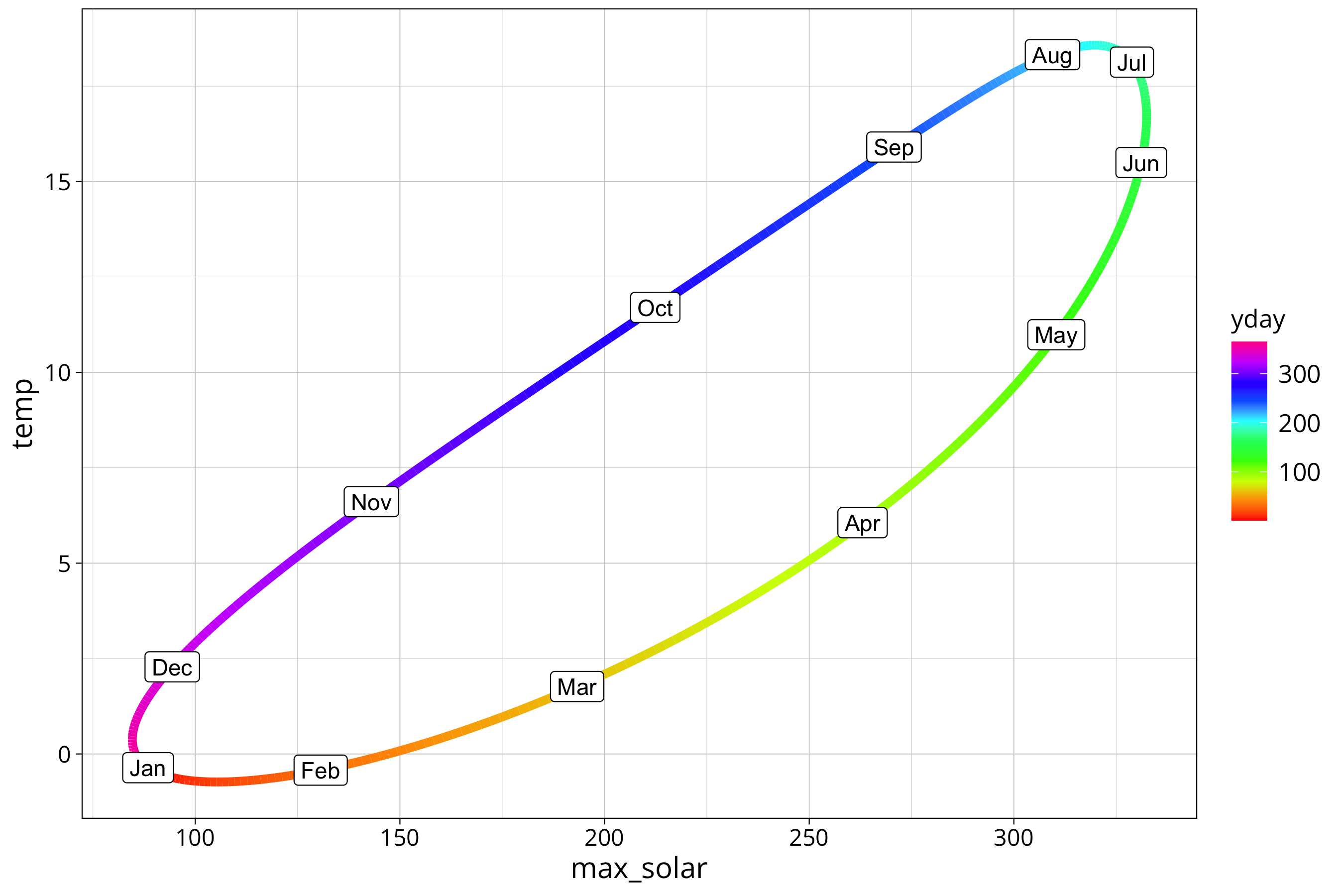

plot of chunk cycle plot solar max

The plot shows the hysteresis between solar radiation and air temperature. Higher radiation is not directly translated into higher air temperature. There is a lag between the signals. We see that the cooling off phase in autumn is more direct as the warming in spring. The curve is more straight from August to December and takes a bit of a detour between January and July.

Here we have the same picture for the mean radiation:

year_prediction %>%
  ggplot() + 
  aes(y=temp, x=mean_solar, col=yday) +
  scale_color_gradientn(colours = rainbow(10), na.value=NA) +
  geom_path(lwd=2) +
  geom_point(aes(col=first_of_month), size=4) +
  geom_label(aes(label=month.abb[first_of_month]), col="black")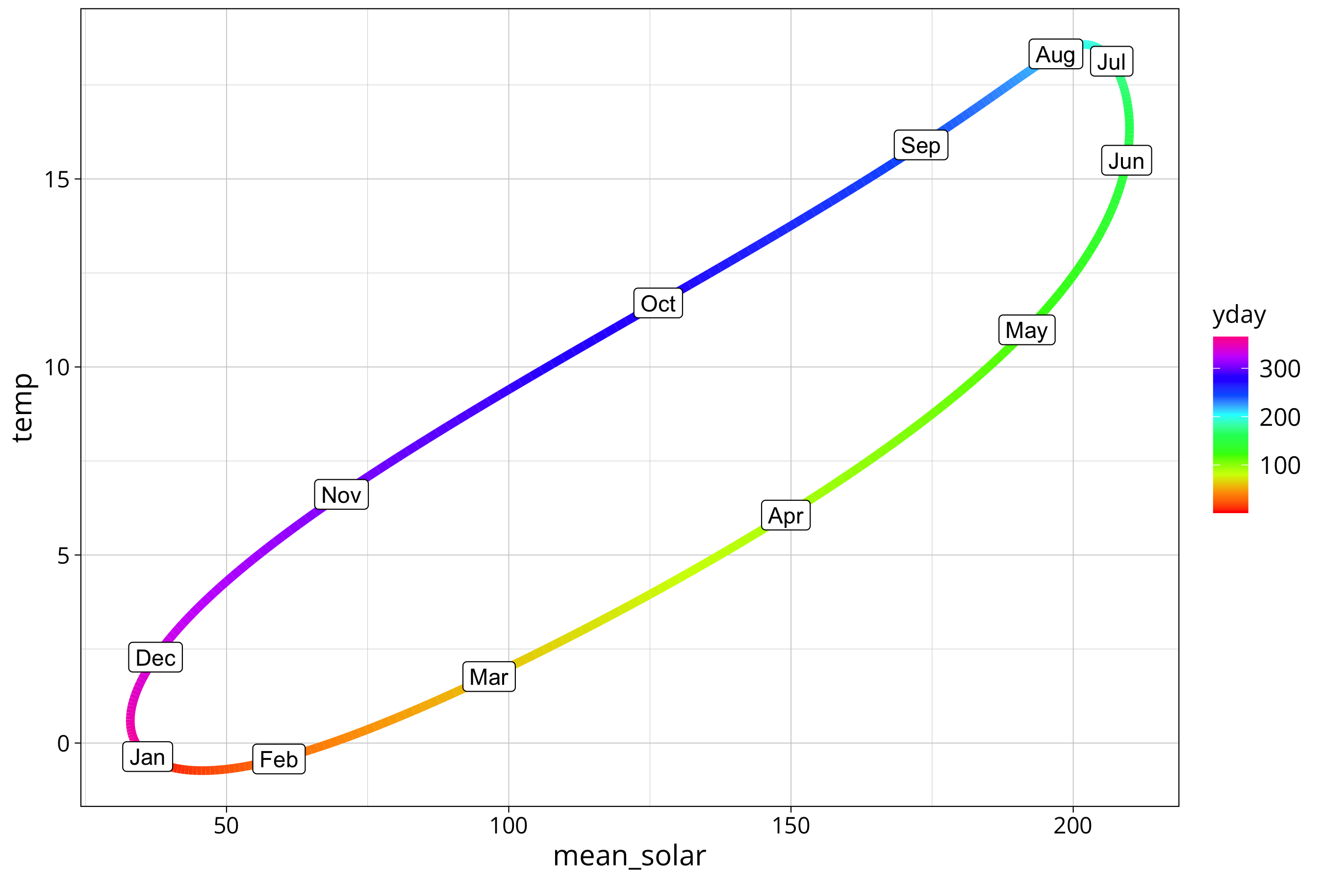

plot of chunk cycle plot solar mean

Note that in this type of plot a perfect 90 degree phase shift between the two signals would create a perfect circle. A total sync of the phase would create a line (100% correlation between the signals). Every phase shift in between creates an oval. Since one of our signals is combined from 3 different frequencies the oval get’s flattened on one side.