Runoff simulations in urban areas necessarily need to include buildings as obstacles for surface runoff. Since most digital elevation models (dem) have buildings and vegetation digitally removed we have to add the buildings back in. Of course you could use a digtial surface model (dsm) which includes vegetation and buildings. But vegetation is a completely different obstacle that has to be treated differently than buildings. So it would be nice to only have buildings in the height map.

Our approach here will be to download a dem from the Geobasis NRW service of the German state Nordhrein Westfalen (NRW) and add buildings from another data product they provide.

Let’s start with loading the necessary packets:

library(tmap)      # for plotting maps
library(stringr)   # for string manipulations
library(sf)        # for working with shapefiles
library(raster)    # for raster math
library(plyr)      # for apply functions
library(dplyr)     # for the pipe operator
library(osmdata)   # for getting locations of landmarks
library(units)     # used by osmdata
library(rayshader) # to render 3d scenes

get bbox for location

In order to download data we will need a bounding box for the data query. We will work with a location that in 2021 got sadly famous for a very deverstating flood event.

We will add a radius of 100 meters around the central location and take that as a bounding box.

# define coordinate systems that we will be using
UTM_crs <- st_crs(25832)

# set the location with UTM coordinates
location <- st_point(c(339021.64, 5584350.34)) %>% st_sfc(crs = UTM_crs)

# add a buffer zone around the central location
area <- location %>% st_buffer(dist = set_units(100, "m"))

# calculate bounding box of buffer zone
bbox_UTM  <- area %>% st_bbox() %>% round() 

# create a text string that we can use later
bbox_UTM_txt <- bbox_UTM %>% paste(collapse = ",")

To get an impression of the location here you have a code and screenshot to produce an interactive openstreetmap plot of the location:

tmap_mode("view")
tm_basemap(leaflet::providers$OpenStreetMap) +
  tm_shape(area) +
  tm_borders()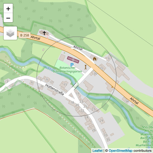

plot of chunk plot location on openstreetmap

download dem

To download the dem we use the raster() function of the raster package. More about that process you can learn in the tutorial about wcs data.

dem <- raster(str_glue("https://www.wcs.nrw.de/geobasis/wcs_nw_dgm?VERSION=2.0.1&SERVICE=wcs&REQUEST=GetCoverage&COVERAGEID=nw_dgm&FORMAT=image/tiff&SUBSET=x({bbox_UTM$xmin},{bbox_UTM$xmax})&SUBSET=y({bbox_UTM$ymin},{bbox_UTM$ymax})&SCALEFACTOR=1&SUBSETTINGCRS=EPSG:25832"))

names(dem) <- "elevation"

download buildings shape

To download shapefiles we use the read_sf() function of the sf package. More about this you can learn in the tutorial about wfs data.

buildings <- read_sf(str_glue("https://www.wfs.nrw.de/geobasis/wfs_nw_alkis_vereinfacht?Service=WFS&REQUEST=GetFeature&VERSION=2.0.0&TYPENAMES=ave:GebaeudeBauwerk&COUNT=10000&BBOX={bbox_UTM_txt},urn:ogc:def:crs:EPSG::25832"))

Let’s plot dem and buildings together:

tmap_mode("plot")
tm_shape(dem) +
  tm_raster() +
  tm_shape(buildings) +
  tm_borders()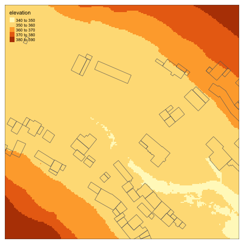

plot of chunk building shapes

calculate elevation of building rooftops

The actual height of the building is not that relevant for the flow simulation. It only has to be a height that effectively blocks the flow path. Therefore we will give all buildings the same height of 8 meters. We will also make the rooftops flat since we don’t have any information about the roof types and roofs usually are drained into the sewer system.

Where buildings are located at a slope we will give the building a height of 8 meters above the highest point of the terrain they are standing on. Therefore we first calculate the maximum height at location of building:

buildings$maxheight <- raster::extract(dem, buildings, fun=max)[,1]

Calculate rooftop height as 8 meters above the maximal height:

buildings$buildheight = buildings$maxheight + 8

Plot the results:

tmap_mode("plot")
tm_shape(buildings) +
  tm_fill(col = "maxheight")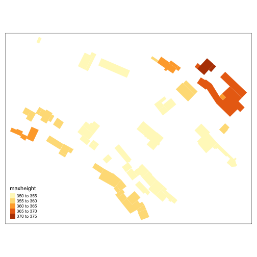

plot of chunk plot rooftop height

rasterize shapefile

We then rastarize the buildings and merge it with the dem:

buildings_dem <- raster::rasterize(buildings, dem, "buildheight", fun=max, background=NA) 
dem_plus_buildings <- max(dem, buildings_dem, na.rm=T)

3d plot

To get a 3d view of the resulting elevation model we use the rayshader package:

dem_plus_buildings_mat <- raster_to_matrix(dem_plus_buildings)

dem_plus_buildings_mat %>%
  sphere_shade(texture = "desert") %>%
  add_shadow(ray_shade(dem_plus_buildings_mat, zscale = 1), 0.5) %>%
  add_shadow(ambient_shade(dem_plus_buildings_mat), 0.7) %>%
  plot_3d(dem_plus_buildings_mat, zscale = 1, fov = 5, theta = 45, zoom = 0.65, phi = 30, windowsize = c(1400, 1000))

Sys.sleep(0.2)
render_snapshot()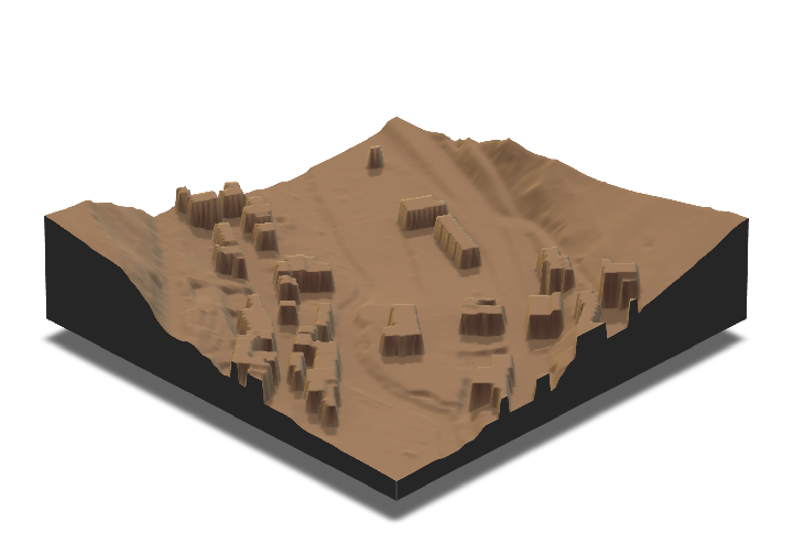

plot of chunk 3d plot

disaggregate to get higher resolution

The dem has a resolution of 1m x 1m. With disaggregation we can render that down to for example 25cm x 25cm. This enables much sharper edges for the buildings.

dem_4x <- disaggregate(dem, fact=4, method='bilinear')
buildings_dem_4x <- rasterize(buildings, dem_4x, "buildheight", fun=max, background=NA) 
dem_plus_buildings_4x <- max(dem_4x, buildings_dem_4x, na.rm=T)
dem_plus_buildings_mat_4x <- raster_to_matrix(dem_plus_buildings_4x)

dem_plus_buildings_mat_4x %>%
  sphere_shade(texture = "desert") %>%
  add_shadow(ray_shade(dem_plus_buildings_mat_4x, zscale = 1/4), 0.5) %>%
  add_shadow(ambient_shade(dem_plus_buildings_mat_4x), 0.75) %>%
  plot_3d(dem_plus_buildings_mat_4x, zscale = 1/4, fov = 5, theta = 45, zoom = 0.65, phi = 30, windowsize = c(1400, 1000))

Sys.sleep(0.2)
render_snapshot()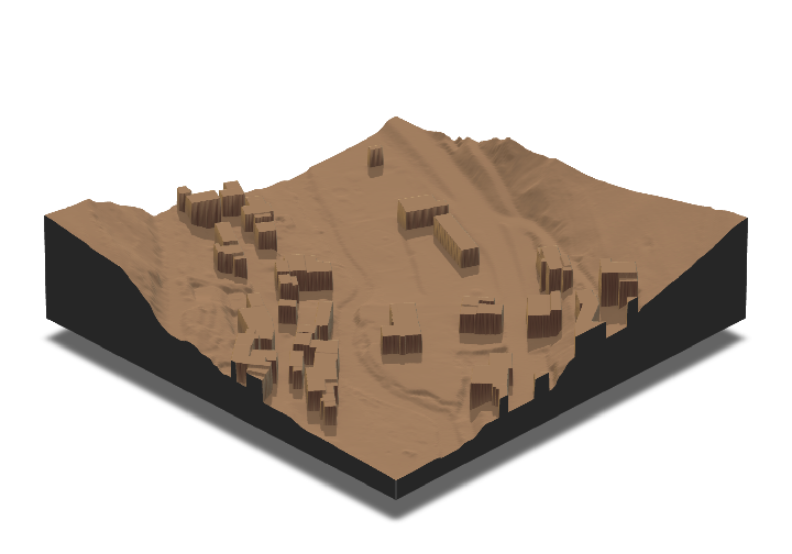

plot of chunk disaggregated 3d plot

The corners of the buildings are much sharper now.